Understanding Phase Relationships in Constructive and Destructive Interferences

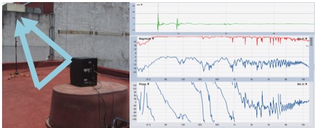
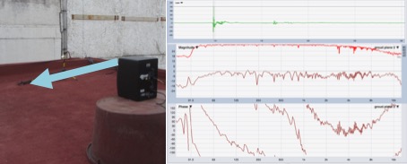
If a tree falls in the forest and nobody is there to hear it, does it make a sound? If an engineer walks between two loudspeaker systems and says it sounds “phase-y,” is there really a “phase issue”? What does that even mean?? In the world of audio, music results from the amazing amalgamation when science and art combine together. Descriptive terms often define subjective experiences whose origin can either be proven or disproven objectively using tools such as measurement devices that utilize dual-channel FFTs (Fast-Fourier Transforms). The problem that we audio engineers face when dealing with the physics of sound is that we deal with wavelengths in orders of magnitude from the size of a coin to the size of a building (see my blog on acoustics here for more info). How two different waveforms interact depends on many factors including frequency, amplitude, and phase. Not to mention what medium they are traveling through, what atmospheric conditions exist, and more…The point being is that there isn’t a one-size-fits-all answer because most of the time the answer is frequency and phase-dependent. When two correlated audio signals at the same frequency combine, do they really create 6dB of gain from summation? Well, the answer is…it depends.

Back To The Basics

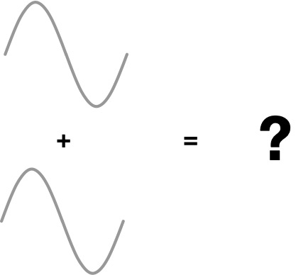
Before we go any further, let’s talk about what comprises a complex waveform. In 1807, Jean-Baptiste Fourier wrote in his memoir On the Propagation of Heat in Solid Bodies [1] his theory that any complex waveform can be broken down into many component sine waves that, when reconstructed, form the original waveform. This theory would be known as a Fourier Transform [1]. The Fourier Transform forms the basis of the math that allows us to perform the signal processing in dual-channel Fast-Fourier Transforms, which in turn allow us to take data in the time domain and analyze it in the frequency domain. Without going too far down the rabbit hole of FFTs, let’s take what Jean-Baptiste Fourier has taught us about complex waveforms and know that by analyzing examples from simple sine waves, we can apply the same concepts to the behavior of more complex waveforms, but layered together to create an end result. The question then becomes what happens when you layer these simple sine waves together?

Let’s narrow our focus from complex waveforms to sine waves and first define some basic terminology such as constructive and destructive interference. When two correlated waveforms, whether it be discrete values of an electronic signal or a mathematical representation of air oscillations, combine together to create an increase in amplitude of the combining individual waveforms, it is known as constructive interference.

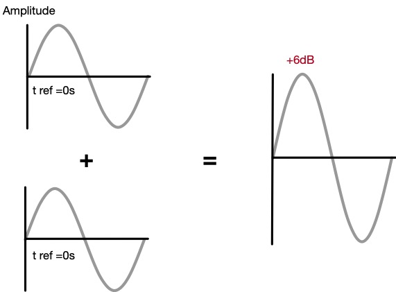
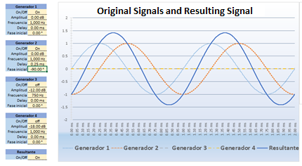
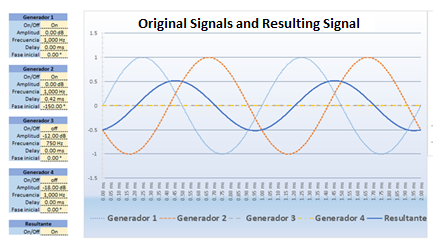
Figure A

When the two correlated signals combine to form a decrease in amplitude, this is called destructive interference. In the worst-case scenario, with enough offset in time or a polarity reversal of one of the individual waveforms, the waveform results in complete cancellation.

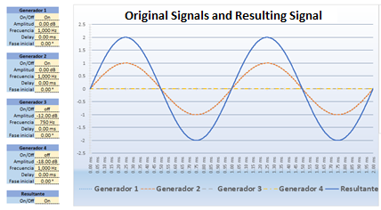
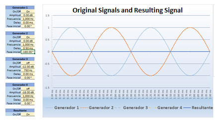
Figure B

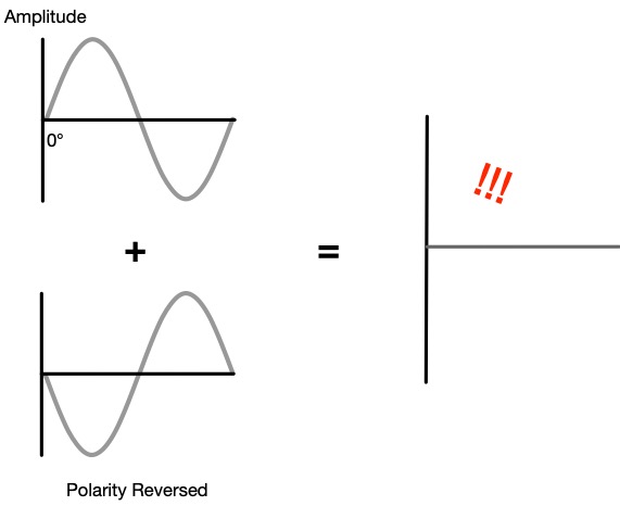
Figure C

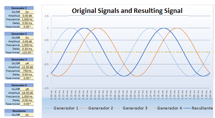
What’s important to note in these graphics is that both waveforms have the exact same frequency and amplitude (for the sake of this example 1000 Hz or 1kHz), but the difference is their offset in time or polarity. In Figure A, both waves start at the same time with the same amplitude so that the sum results in constructive interference which we audibly perceive as a +6dB increase in amplitude. In Figure B one wave starts at time zero while the other starts with a 0.0005s offset in time, this results in a phase offset of 180 degrees (don’t worry we will get into this more) which results in theoretical perfect cancellation of the two waveforms. Similarly in Figure C, the two waveforms start at the same time zero, but one wave has a polarity reversal where the one form starts at the crest of the wave and the other starts at the trough of the wave. This also results in a theoretical perfect cancellation, but it is important to note that a polarity reversal does not involve any offset in time. It is a physical (or electronic) “flip” of the waveform that can result from situations like having the + or – leads on a cable going to an opposite terminal on an amplifier, or pins 2 and 3 on one side of an XLR reversed compared to the other side, or the engagement of a polarity reversal switch on a console, etc. It is also important to point out that we are talking about the effects of time offset versus a polarity reversal in simple sine waves. In these cases, the destructive effects cause the same result, but as soon as we talk about complex waveforms we can definitely tell the difference between the two because there is more than one frequency involved.

So we have reviewed the basics of how waves interfere with one another, but we still haven’t explained what phase actually is. We have only talked about what happens when two waves combine and in what circumstances they will do so constructively or destructively.

In The Beginning, There Was A Circle

In order to really understand what we are talking about when we are talking about phase, we are going to dive even further back into our basic understanding of sound. Not just sound, but how we represent a wave in mathematical form. Recall that sound, in and of itself, is the oscillation of molecules (typically) air traveling through a medium and for us humans we perceive the oscillations moving the organs in our ears at rates between 20Hz to 20,000Hz (if we are lucky). We represent the patterns of this movement in mathematical form as sine waves at different frequencies (remember what Fourier said earlier about complex waveforms?). Because of the cyclical nature of these waves, i.e. the wave repeats itself after a given period, one period of the wave can be thought of as a circle unwound across a graph.

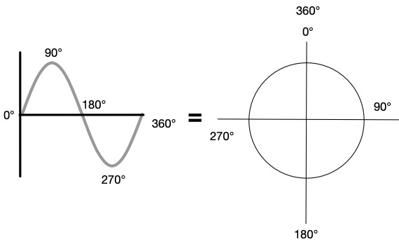
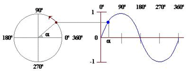
A sine wave can be thought of as an unwound circle

This concept blew my mind when I first put these two things together. The magic behind this is that many cyclical behaviors in nature from light to quantum particles can be represented through wave behavior! WOW! So now that we know that a wave is really just a circle pulled apart across the period of a given frequency (more on that to come!), we can break up a circle in terms of degrees or radians (for math and formal scientific calculations). Conversely, we can indicate what position at a particular point along that waveform is in terms of degrees or radians along the circle. This is the phase at that given position. In the analog world, we talk about phase in relation to time because it took some amount of time, however small, for the waveform to get to that particular position. So how do we figure out what the phase is at a given time for a given frequency sine wave? Time for some more math!

Three Important Formulas in Sound

If you can imprint in your brain three formulas that can be applied to sound for the rest of your life, I highly recommend remembering these three (though we will only really go into two in this blog):

1/T=f or 1/f=T

1/period of a wave in seconds (s) = frequency (in cycles per second or Hertz (Hz))

or

1/frequency of a wave (Hz) = period of a wave (in seconds)

λ =c/f

wavelength (feet or meters) = speed of sound (feet per second ft/s or meters per second m/s) / frequency (Hz)

**must use the same units of distance on both sides of the equation!! (feet or meters)**

V=IR (Ohm’s Law (DC version))

Voltage (Volts) =Current (Amperes) x Resistance (Ohms)

The first equation is very important because it shows the reciprocal relationship between the period of a wave (the overall duration in time for one cycle to complete) to the frequency of the wave (in cycles per second or Hertz). Let’s go back to the example from before of the 1,000Hz sine wave. Using one form of the first equation T=1/f we find that for a 1,000Hz sine wave:

1/1,000 Hz = 0.001 s

The period of a 1,000Hz sine wave is 0.001s or 1 millisecond (1ms). We can visualize this as the amount of time it takes to complete one full cycle and travel from 0 to 360 degrees around the 1,000Hz circle as 1ms or 0.001s.

1,000Hz sine wave with a period of 1ms

The thing is, in most scenarios, phase doesn’t have much meaning to us unless it’s in relation to something else. Time doesn’t have much meaning to us unless it’s in relation to another value. For example, we aren’t late for a meeting unless we had to be there at noon and it is now 2:00 pm. If the meeting had no time reference, would we ever be late? Similarly, a signal by itself can start at any given position in-phase/time and it’s just the same signal…later in time…But if you combine two signals, one starting at one time and the other offset by some value in time, now we start to have some interaction.

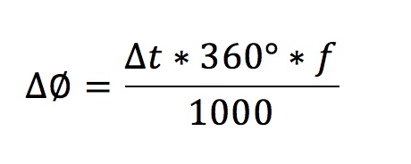
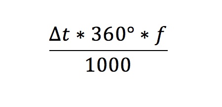
Since we now understand phase as a value for a position in time along the period of a waveform, we can do a little math magic to figure out what the phase offset is based on the time offset between two waveforms. Let’s take our 1,000Hz waveform and now copy it and add the two together, except this time one of the waveforms is offset by 0.0005s or 0.5ms. If we take the ratio of the time offset divided by the period of the 1,000Hz waveform (0.001s or 1ms) and multiply that by 360 degrees, we get the phase offset between the two signals in degrees.

(360 degrees )*((time offset in seconds / period of wave in seconds))

(360)*((0.0005)(0.001))=180 degrees

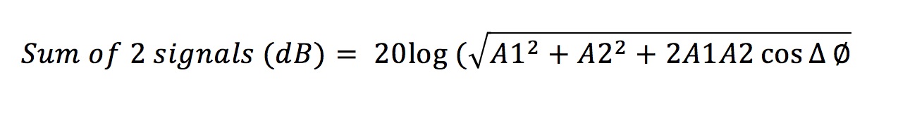
That means that when two copies of the same correlated 1,000Hz signals are offset by 0.5ms they are offset by 180 degrees! If you combined these two at equal amplitude you would get destructive interference resulting in near-perfect cancellation! Knowing the frequency of interacting waves is only part of the picture. We can see that the phase relationship between correlated signals is equally important to understanding whether the interference will be constructive or destructive. It should be noted here that in all these examples we are talking about combining correlated signals of equal amplitude. If we have an amplitude or level offset between the signals, that will affect the summation as well! So how do we know whether a phase offset or offset in time will be destructive or constructive? Is it arbitrary? The answer is: it depends on the frequency!

Understanding Phase In Relation to Frequency

Remembering our 1,000Hz sine wave has a period of 1ms based on using the formula for the reciprocal relationship between frequency and period, let’s find the period of a 100Hz waveform:

1/f=T

1/100=0.01s or 10ms

That means the period of a 100Hz wave is ten times longer than the period of a 1,000Hz wave! A time offset between two copies of the same frequency wave at equal amplitude will have phase offsets dependent on their frequency because of their different periods. For example, the 0.5ms offset between two 1,000 Hz waveforms results in a 180 degree offset, but if we do the math for the same offset in time between two 100Hz waves,

(360 degrees)(0.0005s/0.01s)=18 degrees

That’s only an offset of 18 degrees! Will an 18 degree offset of two correlated sine waves at 100Hz have a constructive or destructive effect? (Remember for the sake of simplicity we are assuming equal amplitude for these examples). In order to understand this, let’s look back at a basic drawing of a sine wave:

Figure D

So here is the really cool part: much like we can use a sine wave or a circle to represent the cyclical nature of the period of a wave, we can also use a sine wave to describe the relationship between identical waveforms as well! Or rather we can use a sine wave/circle to describe the phase relationship between the two waves as an offset between the two waveforms because the effects are also cyclical in nature! We just went through the math of how different time offsets equate to a different phase relationship depending on frequency, so if you were to look at the effects of a time offset across a spectrum of frequencies, you would see a cyclical waveform of that phase response itself as it changes depending on the frequency! It’s like a sine wave inception!!

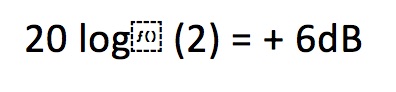
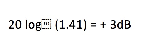
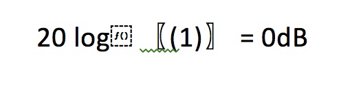
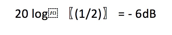
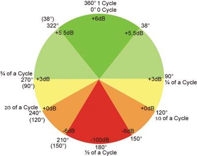
In Figure D we see the markings for phase along the waveform or unwrapped circle as we learned earlier. We have also learned that these positions in time will change depending on the period/frequency of the waveform. Visually we can see as you approach 90 degrees on the sine wave, the slope of the wave increases up until roughly the 60-degree point where it begins to “flatten” out. This means if we were interpreting this as the phase response between two correlated signals, the resultant wave would still be increasing in amplitude. The summation of two identical, correlated waveforms at this offset will still result in addition. From +6dB when there is 0 degree offset since the two waveforms begin at the same time, up to 3dB at 90 degrees. Yet after 90 degrees, the slope begins to decrease, indicating that when we combine two identical waveforms with an offset in this range we begin losing summation and enter destructive interference until we reach 180 degrees, which results in theoretical perfect cancellation. As we continue our journey along the period of this waveform, we continue with destructive interference to a lessening degree until the trough of the waveform “flattens” out again at 270 degrees where we again have reached +3dB summation. After 270 degrees we increase in amplitude until we reach 360 degrees at which point we have made it all the way around the circle and the entire period of the waveform to 6dB of summation again. Merlijn Van Veen has a great graphic of the “wheel of phase” on his website that offers a visual representation of the relative gain (in decibels) between two identical, correlated signals as indicated by their phase relationship [2].

What this means is that whether two correlated signals will combine to form a destructive or constructive resultant waveform will depend on their frequency, amplitude, and phase relationship to one another. It’s easy to extrapolate that as you start talking about complex waveforms interacting, you are managing multiple frequencies at different amplitudes so describing the phase relationships between the interactions becomes more and more convoluted.

And Now Comb Filters

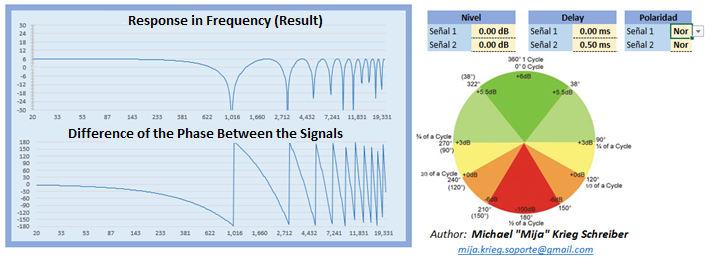
So now that we have come back from this world of mathematical representations of real-world behaviors, how can we actually apply this to the real world? Recall from the beginning of this blog the example of the engineer walking between two loudspeakers and declaring it to sound “phase-y”. Here is where we can finally understand what the engineer is hearing by using our new understanding of what phase actually means to describe the audible peaks and dips of the comb filter. A comb filter results from the combination of two wide-spectrum signals with some offset in the time domain. In fact, any change in level or phase relationship between the two correlated signals will affect the severity of the comb filter. Let’s imagine that the engineer is listening at a position equidistant from the two loudspeakers that are spaced equal distance apart from their acoustic centers and both have fairly wide dispersion patterns. For the sake of relative simplicity, we will make them directional point sources with a pattern wide enough to fully overlap each other. Let’s then imagine that both loudspeakers are playing the same identical broadband pink noise signal to both loudspeakers. With both loudspeakers playing identical signals at identical time, the engineer should hear an additive 6dB of summation from the two signals adding together. If one of the speakers gets pushed back roughly 1.125ft or gets 1ms of time delay added electronically via the DSP, the engineer will hear the resultant comb filter at the listening position. There will be a 1,000Hz spacing between nulls of this comb filter. We can figure that out using two of our handy physics equations from earlier. For the time offset of 1ms:

f=1/T so 1/0.001s=1,000Hz

And if we physically pushed back the speaker about 1ft, we can use the formula for wavelength to find the frequency:

Wavelength = speed of sound / frequency

or in this case, by doing some algebra we can rewrite that as:

Frequency = speed of sound / wavelength

The speed of sound at “average sea level”, which is roughly 1 atmosphere or 101.3 kiloPascals [3]), at 68 degrees Fahrenheit (20 degrees Celsius), and at 0% humidity is approximately 343 meters per second or approximately 1,125 feet per second [4] (see more about this in my blog on Acoustics). If we calculate this using the speed of sound in ft/s since our measurement of the displacement is in feet, we again get the resultant comb filter spacing of 1,000Hz:

1,125 ft/s / 1.125ft = 1,000Hz

Both equations allow us to predict or explain anomalies that we hear. These equations allow us to understand how to calculate the general behavior of comb filters! Now we can take this one step further by talking about subwoofer spacing.

There is a common trope in live sound of spacing subs within a “quarter-wavelength apart”. Using our knowledge of how the phase relationship between two correlated waveforms will be frequency-dependent, we can understand on a basic level (without taking into account room acoustics and other complex acoustical calculations) how if you take a critical frequency say of 60Hz and use that as your “frequency of interest” if you stay within 60 degrees of time offset between the two subwoofers, they will still result in summation to some degree at that frequency.

The truth is that understanding the interactions of complex waveforms involves not just doing these calculations based on one frequency of interest. We are dealing with complex waveforms composed of many different frequencies all in orders of magnitude different from one another with behavior that changes depending on what frequency bandpass you are talking about. Not to mention also including the interactions of room acoustics, atmospheric conditions, and other external factors. There is no one-size-fits-all solution, but by breaking down complex waveforms into their component sine waves and using the advancements in technology and analysis tools to crunch the numbers for us, we can use all the tools at our disposal to see the bigger picture of what’s happening when two waveforms interact.

Endnotes:

[1] https://www.aps.org/publications/apsnews/201003/physicshistory.cfm

[2] https://www.merlijnvanveen.nl/en/study-hall/169-displacement-is-key

[3] (pg. 345) Giancoli, D.C. (2009). Physics for Scientists & Engineers with Modern Physics. Pearson Prentice Hall.

[4] http://www.sengpielaudio.com/calculator-airpressure.htm

Resources:

American Physical Society. (2010, March). This Month in Physics History March 21, 1768: Birth of Jean-Baptiste Joseph Fourier. APS News. https://www.aps.org/publications/apsnews/201003/physicshistory.cfm

Everest, F.A. & Pohlmann, K. (2015). Master Handbook of Acoustics. 6th ed. McGraw-Hill Education.

Lyons, R.G. (2011). Understanding Digital Signal Processing. 3rd ed. Prentice-Hall: Pearson Education.

van Veen, M. (2019). Displacement is Key. Merlijn van Veen. https://www.merlijnvanveen.nl/en/study-hall/169-displacement-is-key